Sesión 12

Estimación de parámetros en redes bayesianas

Objetivos:

• Obtener los parámetros de máxima verosimilitud para redes Bayesianas.

• Obtener los parámetros MAP para redes Bayesianas.

Referencias:

• Probabilistic Graphical Models: Principles and Techniques, By Daphne Koller and Nir Friedman. Ch. 17.

1. Introducción

Una vez que la estructura de una red bayesiana está definida, el siguiente paso es aprender sus parámetros, es decir, las probabilidades que conforman las Conditional Probability Distributions (CPDs) de cada nodo.

Suponemos que disponemos de un conjunto de datos completamente observados:

\[ \mathcal{D} = \{d_1, d_2, \ldots, d_N\} \]

Cada instancia contiene un valor para cada nodo de la red.

El objetivo del aprendizaje de parámetros es encontrar los valores de las probabilidades que mejor explican los datos observados.

Este problema aparece frecuentemente cuando:

• un experto puede definir la estructura, pero no los valores numéricos de las probabilidades,

• queremos ajustar el modelo a datos reales,

• necesitamos estos parámetros como parte de procedimientos más complejos (p. ej., aprendizaje de estructura o aprendizaje con datos incompletos).

Existen dos enfoques principales para estimar parámetros:

1. Estimación por Máxima Verosimilitud (MLE)
2. Estimación Bayesiana (MAP / Dirichlet priors)

1.1 Estimación por Máxima Verosimilitud (MLE)

La idea es simple: elegir los parámetros que hacen más probable el dataset bajo el modelo.

Buscamos: $\( \theta^{*}=\arg\max_\theta P(\mathcal{D}\mid\mathcal{M}(\theta)) \)$

Con datos i.i.d.: $\( P(\mathcal{D}\mid\mathcal{M})=\prod_{m=1}^N P(d_m\mid\mathcal{M}) \)$

MLE solo dice: “ajusta \(\theta\) para que lo que viste en los datos sea lo más probable posible”.

1.1.1. MLE en redes bayesianas discretas

Cada nodo discreto (con o sin padres) genera conteos de sus valores observados.

La verosimilitud es la de una multinomial: multiplicamos la probabilidad de cada valor tantas veces como aparece en el dataset.

Para un nodo con padres \(U\): $\( L(\theta)=\prod_{x,u}\theta_{x\mid u}^{\,N(x,u)} \)$

Para un nodo sin padres: $\( L(\theta)=\prod_x \theta_x^{\,N(x)} \)$

El máximo siempre se obtiene normalizando los conteos:

• Con padres: $\(\hat\theta_{x\mid u}=\frac{N(x,u)}{N(u)}\)$

el estimador de máxima verosimilitud corresponde a la cantidad de muestras consistentes con \(x\) y \(u\) dividido entre la cantidad de muestras consistentes con \(u\).

• Sin padres: $\(\hat\theta_x=\frac{N(x)}{N}\)$

MLE = frecuencias relativas.
Porque para datos categóricos, la multinomial dice: “usa como probabilidad la proporción con la que lo viste ocurrir”.

1.1.2. Ejemplo 1: nodo sin padres

El nodo \(X\) toma valores \(\{0,1,2\}\). En el dataset observamos:

\(X\)	Conteo
0	40
1	35
2	25

Total:
$\(N=40+35+25=100\)$

MLE: $\( \hat\theta_0=\tfrac{40}{100}=0.40,\quad \hat\theta_1=\tfrac{35}{100}=0.35,\quad \hat\theta_2=\tfrac{25}{100}=0.25 \)$

1.1.3. Ejemplo 2: nodo con padres

Supón que \(X\) tiene un padre \(U\). Miramos solo las filas donde \(U=u\):

\(X\)	\(U=u\)	Conteo \(N(x,u)\)
0	u	30
1	u	50
2	u	20

Total dado \(u\):
$\(N(u)=100\)$

MLE: $\( \hat\theta_{0\mid u}=\tfrac{30}{100}=0.30,\quad \hat\theta_{1\mid u}=\tfrac{50}{100}=0.50,\quad \hat\theta_{2\mid u}=\tfrac{20}{100}=0.20 \)$

En ambos casos: frecuencias relativas = parámetros MLE

1.2. Conexión con el .fit() de pgmpy

El método:

.fit de pgmpy implementa exactamente este procedimiento de MLE para redes bayesianas con datos completamente observados.

En este caso vamos a generar un ejemplo de Naive Bayes usando el dataset de vinos y poniendo atención en la estimación de los parámetros mediante MLE.

from pgmpy.models import DiscreteBayesianNetwork
import matplotlib.pyplot as plt
import seaborn as sns
import pandas as pd
import numpy as np

import os
ruta = os.path.join('..', 'data', 'winequality-red.csv')
wine_data = pd.read_csv(ruta, sep=";")

wine_data.shape

(1599, 12)

wine_data.head()

	fixed acidity	volatile acidity	citric acid	residual sugar	chlorides	free sulfur dioxide	total sulfur dioxide	density	pH	sulphates	alcohol	quality
0	7.4	0.70	0.00	1.9	0.076	11.0	34.0	0.9978	3.51	0.56	9.4	5
1	7.8	0.88	0.00	2.6	0.098	25.0	67.0	0.9968	3.20	0.68	9.8	5
2	7.8	0.76	0.04	2.3	0.092	15.0	54.0	0.9970	3.26	0.65	9.8	5
3	11.2	0.28	0.56	1.9	0.075	17.0	60.0	0.9980	3.16	0.58	9.8	6
4	7.4	0.70	0.00	1.9	0.076	11.0	34.0	0.9978	3.51	0.56	9.4	5

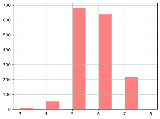
wine_data.quality.value_counts()

quality
5    681
6    638
7    199
4     53
8     18
3     10
Name: count, dtype: int64

# histograma de la variable objetivo
wine_data["quality"].hist(
                        bins=5,
                        color="red",
                        alpha=0.5,
                        width=0.5)

<Axes: >

# target
target = "quality"

# vars independientes
variables = [col for col in wine_data.columns if col != target]

print('Target:', target)
print('Variables independientes:', variables)

Target: quality
Variables independientes: ['fixed acidity', 'volatile acidity', 'citric acid', 'residual sugar', 'chlorides', 'free sulfur dioxide', 'total sulfur dioxide', 'density', 'pH', 'sulphates', 'alcohol']

# pandas qcut
pd.qcut?

Nota: En este ejemplo usamos el mismo número de cuantiles para todas las variables solo para simplificar. En la práctica, cada variable debería discretizarse según su propia distribución (no todas requieren la misma cantidad ni el mismo tipo de cortes).

# Cuantificación de variables numéricas
quantiles = 10
for col in variables:
    wine_data[col] = pd.qcut(wine_data[col], q=quantiles, labels=range(1, 11))
wine_data.head()

	fixed acidity	volatile acidity	citric acid	residual sugar	chlorides	free sulfur dioxide	total sulfur dioxide	density	pH	sulphates	alcohol	quality
0	4	9	1	3	4	4	5	8	9	3	2	5
1	5	10	1	8	9	9	8	6	3	7	4	5
2	5	10	2	6	8	6	7	6	4	6	4	5
3	10	1	10	3	4	7	8	8	2	4	4	6
4	4	9	1	3	4	4	5	8	9	3	2	5

wine_data['quality'].value_counts().sort_index()

quality
3     10
4     53
5    681
6    638
7    199
8     18
Name: count, dtype: int64

wine_data['volatile acidity'].value_counts().sort_index()

volatile acidity
1     175
2     161
3     145
4     171
5     164
6     148
7     161
8     159
9     157
10    158
Name: count, dtype: int64

# Red Bayesiana
wine_model_naive = DiscreteBayesianNetwork([
    ('quality', 'fixed acidity'),
    ('quality', 'volatile acidity'),
    ('quality', 'citric acid'),
    ('quality', 'residual sugar'),
    ('quality', 'chlorides'),
    ('quality', 'free sulfur dioxide'),
    ('quality', 'total sulfur dioxide'),
    ('quality', 'density'),
    ('quality', 'pH'),
    ('quality', 'sulphates'),
    ('quality', 'alcohol'),
])

Aquí dejo la documentación acerca de plotting models de pgmpy.

# Dibujar red con daft 
# ojo porque aquí necesitamos instalar daft: https://docs.daft-pgm.org/en/latest/

model_plot = wine_model_naive.to_daft(
    node_pos="shell",
    pgm_params={"observed_style": "outer", "grid_unit": 5}
)
model_plot.render()

---------------------------------------------------------------------------
ImportError                               Traceback (most recent call last)
Cell In[13], line 4
      1 # Dibujar red con daft
      2 # ojo porque aquí necesitamos instalar daft: https://docs.daft-pgm.org/en/latest/
      3 
----> 4 model_plot = wine_model_naive.to_daft(
      5     node_pos="shell",
      6     pgm_params={"observed_style": "outer", "grid_unit": 5}
      7 )

File ~/checkouts/readthedocs.org/user_builds/modelos-graficos-probabilisticos/envs/v2026/lib/python3.13/site-packages/pgmpy/base/DAG.py:1229, in DAG.to_daft(self, node_pos, latex, pgm_params, edge_params, node_params, plot_edge_strength)
   1227     from daft import PGM
   1228 except ImportError as e:
-> 1229     raise ImportError(
   1230         f"{e}. Package `daft` is required for plotting probabilistic graphical models.\n"
   1231         "Please install it using: pip install daft-pgm\n"
   1232         "Documentation: https://docs.daft-pgm.org/en/latest/"
   1233     ) from None
   1235 # Check edge strength existence if plotting is requested
   1236 if plot_edge_strength:

ImportError: No module named 'daft'. Package `daft` is required for plotting probabilistic graphical models.
Please install it using: pip install daft-pgm
Documentation: https://docs.daft-pgm.org/en/latest/

# Train y test
train_df = wine_data.sample(frac=0.8, random_state=42)
test_df = wine_data.drop(train_df.index)
train_df.shape, test_df.shape

((1279, 12), (320, 12))

• nota que aquí usamos el .fit() de pgmpy para estimar los parámetros de la red bayesiana usando MLE.

# Entrenamos
wine_model_naive.fit(train_df)

INFO:pgmpy: Datatype (N=numerical, C=Categorical Unordered, O=Categorical Ordered) inferred from data: 
 {'fixed acidity': 'O', 'volatile acidity': 'O', 'citric acid': 'O', 'residual sugar': 'O', 'chlorides': 'O', 'free sulfur dioxide': 'O', 'total sulfur dioxide': 'O', 'density': 'O', 'pH': 'O', 'sulphates': 'O', 'alcohol': 'O', 'quality': 'N'}

<pgmpy.models.DiscreteBayesianNetwork.DiscreteBayesianNetwork at 0x120a7b610>

wine_model_naive.check_model()

True

# CPDs estimadas -- target
print(wine_model_naive.get_cpds(target))

+------------+------------+
| quality(3) | 0.00547303 |
+------------+------------+
| quality(4) | 0.03362    |
+------------+------------+
| quality(5) | 0.433151   |
+------------+------------+
| quality(6) | 0.388585   |
+------------+------------+
| quality(7) | 0.12588    |
+------------+------------+
| quality(8) | 0.0132916  |
+------------+------------+

# train value counts -- target
train_df[target].value_counts().sort_index()

quality
3      7
4     43
5    554
6    497
7    161
8     17
Name: count, dtype: int64

# CPDs estimadas -- alcohol | target
print(wine_model_naive.get_cpds("alcohol"))

+-------------+---------------------+-----+----------------------+
| quality     | quality(3)          | ... | quality(8)           |
+-------------+---------------------+-----+----------------------+
| alcohol(1)  | 0.14285714285714285 | ... | 0.0                  |
+-------------+---------------------+-----+----------------------+
| alcohol(2)  | 0.0                 | ... | 0.0                  |
+-------------+---------------------+-----+----------------------+
| alcohol(3)  | 0.0                 | ... | 0.0                  |
+-------------+---------------------+-----+----------------------+
| alcohol(4)  | 0.2857142857142857  | ... | 0.058823529411764705 |
+-------------+---------------------+-----+----------------------+
| alcohol(5)  | 0.14285714285714285 | ... | 0.058823529411764705 |
+-------------+---------------------+-----+----------------------+
| alcohol(6)  | 0.0                 | ... | 0.0                  |
+-------------+---------------------+-----+----------------------+
| alcohol(7)  | 0.2857142857142857  | ... | 0.0                  |
+-------------+---------------------+-----+----------------------+
| alcohol(8)  | 0.14285714285714285 | ... | 0.17647058823529413  |
+-------------+---------------------+-----+----------------------+
| alcohol(9)  | 0.0                 | ... | 0.23529411764705882  |
+-------------+---------------------+-----+----------------------+
| alcohol(10) | 0.0                 | ... | 0.47058823529411764  |
+-------------+---------------------+-----+----------------------+

pd.DataFrame(
    data=wine_model_naive.get_cpds("alcohol").values,
    columns=[f"{target}_{i}" for i in range(3, 9)],
    index=[f"alcohol_{i}" for i in range(1, 11)]
)

	quality_3	quality_4	quality_5	quality_6	quality_7	quality_8
alcohol_1	0.142857	0.209302	0.184116	0.112676	0.012422	0.000000
alcohol_2	0.000000	0.023256	0.263538	0.106640	0.006211	0.000000
alcohol_3	0.000000	0.116279	0.054152	0.030181	0.000000	0.000000
alcohol_4	0.285714	0.116279	0.146209	0.094567	0.037267	0.058824
alcohol_5	0.142857	0.093023	0.106498	0.098592	0.074534	0.058824
alcohol_6	0.000000	0.069767	0.084838	0.098592	0.055901	0.000000
alcohol_7	0.285714	0.069767	0.054152	0.118712	0.111801	0.000000
alcohol_8	0.142857	0.139535	0.055957	0.104628	0.186335	0.176471
alcohol_9	0.000000	0.139535	0.032491	0.150905	0.248447	0.235294
alcohol_10	0.000000	0.023256	0.018051	0.084507	0.267081	0.470588

predictions = wine_model_naive.predict(test_df.drop(columns=[target]))

predictions

	fixed acidity	volatile acidity	citric acid	residual sugar	chlorides	free sulfur dioxide	total sulfur dioxide	density	pH	sulphates	alcohol	quality
1	5	10	1	8	9	9	8	6	3	7	4	5
8	5	7	2	3	4	3	2	6	7	4	2	5
13	5	7	6	1	10	3	4	7	4	10	1	5
14	7	8	4	10	10	10	10	9	2	10	1	5
20	7	1	9	2	5	9	8	6	8	2	2	5
...	...	...	...	...	...	...	...	...	...	...	...	...
1569	1	5	4	3	1	6	5	1	9	4	9	6
1570	1	2	10	5	10	7	5	1	7	10	10	7
1573	1	7	4	7	4	6	7	2	10	7	10	6
1583	1	4	6	4	4	10	10	3	6	5	4	5
1595	1	6	3	5	2	10	7	2	10	8	8	7

320 rows × 12 columns

predictions['quality'].values == test_df['quality'].values

array([ True, False,  True,  True, False,  True,  True, False, False,
        True,  True,  True, False, False,  True,  True,  True,  True,
        True,  True,  True, False, False,  True,  True, False,  True,
        True, False,  True,  True,  True,  True, False,  True,  True,
       False,  True,  True,  True,  True,  True, False,  True, False,
       False,  True, False,  True, False, False,  True, False, False,
       False,  True, False,  True, False, False, False,  True,  True,
       False,  True, False, False, False,  True,  True,  True,  True,
        True,  True, False,  True,  True, False,  True,  True, False,
       False,  True,  True,  True,  True,  True, False, False,  True,
       False, False,  True,  True,  True,  True,  True,  True,  True,
        True, False,  True, False,  True, False,  True, False, False,
        True,  True,  True, False,  True, False,  True, False, False,
        True,  True, False, False, False, False,  True,  True,  True,
        True,  True, False,  True,  True,  True, False, False,  True,
       False, False,  True,  True,  True,  True,  True, False,  True,
        True, False,  True,  True,  True, False,  True, False,  True,
       False,  True, False,  True,  True,  True,  True,  True, False,
        True, False,  True,  True,  True,  True,  True,  True, False,
        True,  True,  True, False,  True,  True, False,  True,  True,
        True,  True,  True,  True, False,  True, False, False,  True,
        True,  True, False,  True,  True,  True,  True,  True,  True,
       False,  True,  True, False, False,  True,  True, False,  True,
        True,  True,  True, False, False,  True,  True, False,  True,
        True,  True,  True,  True,  True,  True, False,  True,  True,
       False, False,  True, False,  True,  True, False,  True, False,
        True, False,  True,  True, False,  True, False, False,  True,
        True,  True,  True,  True, False,  True,  True,  True, False,
       False, False, False, False,  True, False,  True, False, False,
        True, False,  True,  True,  True,  True, False,  True,  True,
        True, False,  True,  True,  True, False,  True, False, False,
       False,  True,  True, False, False,  True,  True,  True, False,
       False, False,  True, False, False, False,  True,  True,  True,
        True,  True,  True, False, False, False, False,  True,  True,
        True,  True, False,  True,  True,  True,  True,  True,  True,
        True, False,  True,  True, False])

(predictions['quality'].values == test_df['quality'].values).mean()

np.float64(0.63125)

1.3. fit_update

Algo muy interesante del método fit de pgmpy es que permite un ajuste incremental de los parámetros.

¿Qué significa esto?
Que el modelo puede actualizar sus CPDs con nuevos datos sin volver a entrenar desde cero.

Es exactamente la idea de aprendizaje online o incremental: procesar datos que llegan en bloques o secuencias, manteniendo el modelo al día sin reconstruirlo completamente.

Esto es útil cuando:

• El dataset crece con el tiempo.

• Entrenar desde cero sería costoso.

• Queremos modelos que se adapten continuamente.

Aquí está la documentación del método fit_update. ***

---

2. Estimación MAP

2.1. ¿Cómo prevenimos el overfitting?

MLE copia exactamente las frecuencias del dataset. Si el dataset es pequeño o hay combinaciones poco frecuentes (tienden a cero) → las probabilidades quedan extremas y el modelo sobreajusta.

Solución: introducir suavizado mediante regularización / priors (p. ej., Dirichlet). Esto evita ceros, reparte probabilidad antes de ver datos y produce parámetros más estables.

2.1.1 ¿Qué es la prior Dirichlet?

Queremos modelar una distribución multinomial con parámetros \(\bar{\theta} = [\theta_1,\dots,\theta_k]\). Estas \(\theta_i\) son probabilidades, así que deben sumar 1 y ser ≥ 0.

Dirichlet es simplemente una distribución sobre vectores de probabilidad.

2.1.2 ¿Cómo actualiza la Dirichlet con los datos?

Si contamos en los datos reales cuántas veces apareció cada categoría \(i\):

• \(N_i\) = conteos reales

Entonces la actualización posterior es:

\[ \hat\theta_i = \frac{N_i + \alpha_i}{\sum_j (N_j + \alpha_j)} \]

Dirichlet = multinomial suavizada.

Toma las frecuencias reales y les agrega un poquito de evidencia previa para no sobreajustar.

Es exactamente lo que necesitas cuando:

• tienes pocos datos,

• aparecen valores raros,

• quieres evitar probabilidades 0,

• quieres un modelo más generalizable.

from pgmpy.estimators import BayesianEstimator

help(BayesianEstimator)

Help on class BayesianEstimator in module pgmpy.estimators.BayesianEstimator:

class BayesianEstimator(pgmpy.estimators.base.ParameterEstimator)
 |  BayesianEstimator(model, data, **kwargs)
 |
 |  Class used to compute parameters for a model using Bayesian Parameter Estimation.
 |  See `MaximumLikelihoodEstimator` for constructor parameters.
 |
 |  Method resolution order:
 |      BayesianEstimator
 |      pgmpy.estimators.base.ParameterEstimator
 |      pgmpy.estimators.base.BaseEstimator
 |      builtins.object
 |
 |  Methods defined here:
 |
 |  __init__(self, model, data, **kwargs)
 |      Base class for parameter estimators in pgmpy.
 |
 |      Parameters
 |      ----------
 |      model: pgmpy.models.DiscreteBayesianNetwork or pgmpy.models.MarkovNetwork model
 |          for which parameter estimation is to be done.
 |
 |      data: pandas DataFrame object
 |          dataframe object with column names identical to the variable names of the model.
 |          (If some values in the data are missing the data cells should be set to `numpy.nan`.
 |          Note that pandas converts each column containing `numpy.nan`s to dtype `float`.)
 |
 |      state_names: dict (optional)
 |          A dict indicating, for each variable, the discrete set of states (or values)
 |          that the variable can take. If unspecified, the observed values in the data set
 |          are taken to be the only possible states.
 |
 |      complete_samples_only: bool (optional, default `True`)
 |          Specifies how to deal with missing data, if present. If set to `True` all rows
 |          that contain `np.Nan` somewhere are ignored. If `False` then, for each variable,
 |          every row where neither the variable nor its parents are `np.nan` is used.
 |          This sets the behavior of the `state_count`-method.
 |
 |  estimate_cpd(
 |      self,
 |      node,
 |      prior_type='BDeu',
 |      pseudo_counts=[],
 |      equivalent_sample_size=5,
 |      weighted=False
 |  )
 |      Method to estimate the CPD for a given variable.
 |
 |      Parameters
 |      ----------
 |      node: int, string (any hashable python object)
 |          The name of the variable for which the CPD is to be estimated.
 |
 |      prior_type: 'dirichlet', 'BDeu', 'K2',
 |          string indicting which type of prior to use for the model parameters.
 |          - If 'prior_type' is 'dirichlet', the following must be provided:
 |              'pseudo_counts' = dirichlet hyperparameters; a single number or 2-D array
 |               of shape (node_card, product of parents_card) with a "virtual" count for
 |               each variable state in the CPD. The virtual counts are added to the
 |               actual state counts found in the data. (if a list is provided, a
 |               lexicographic ordering of states is assumed)
 |          - If 'prior_type' is 'BDeu', then an 'equivalent_sample_size'
 |               must be specified instead of 'pseudo_counts'. This is equivalent to
 |               'prior_type=dirichlet' and using uniform 'pseudo_counts' of
 |               `equivalent_sample_size/(node_cardinality*np.prod(parents_cardinalities))`.
 |          - A prior_type of 'K2' is a shorthand for 'dirichlet' + setting every
 |            pseudo_count to 1, regardless of the cardinality of the variable.
 |
 |      weighted: bool
 |          If weighted=True, the data must contain a `_weight` column specifying the
 |          weight of each datapoint (row). If False, assigns an equal weight to each
 |          datapoint.
 |
 |      Returns
 |      -------
 |      CPD: TabularCPD
 |          The estimated CPD for `node`.
 |
 |      Examples
 |      --------
 |      >>> import pandas as pd
 |      >>> from pgmpy.models import DiscreteBayesianNetwork
 |      >>> from pgmpy.estimators import BayesianEstimator
 |      >>> data = pd.DataFrame(data={'A': [0, 0, 1], 'B': [0, 1, 0], 'C': [1, 1, 0]})
 |      >>> model = DiscreteBayesianNetwork([('A', 'C'), ('B', 'C')])
 |      >>> estimator = BayesianEstimator(model, data)
 |      >>> cpd_C = estimator.estimate_cpd('C', prior_type="dirichlet",
 |      ...                                pseudo_counts=[[1, 1, 1, 1],
 |      ...                                               [2, 2, 2, 2]])
 |      >>> print(cpd_C)
 |      ╒══════╤══════╤══════╤══════╤════════════════════╕
 |      │ A    │ A(0) │ A(0) │ A(1) │ A(1)               │
 |      ├──────┼──────┼──────┼──────┼────────────────────┤
 |      │ B    │ B(0) │ B(1) │ B(0) │ B(1)               │
 |      ├──────┼──────┼──────┼──────┼────────────────────┤
 |      │ C(0) │ 0.25 │ 0.25 │ 0.5  │ 0.3333333333333333 │
 |      ├──────┼──────┼──────┼──────┼────────────────────┤
 |      │ C(1) │ 0.75 │ 0.75 │ 0.5  │ 0.6666666666666666 │
 |      ╘══════╧══════╧══════╧══════╧════════════════════╛
 |
 |  get_parameters(
 |      self,
 |      prior_type='BDeu',
 |      equivalent_sample_size=5,
 |      pseudo_counts=None,
 |      n_jobs=1,
 |      weighted=False
 |  )
 |      Method to estimate the model parameters (CPDs).
 |
 |      Parameters
 |      ----------
 |      prior_type: 'dirichlet', 'BDeu', or 'K2'
 |          string indicting which type of prior to use for the model parameters.
 |          - If 'prior_type' is 'dirichlet', the following must be provided:
 |              'pseudo_counts' = dirichlet hyperparameters; a single number or a dict containing, for each
 |               variable, a 2-D array of the shape (node_card, product of parents_card) with a "virtual"
 |               count for each variable state in the CPD, that is added to the state counts.
 |               (lexicographic ordering of states assumed)
 |          - If 'prior_type' is 'BDeu', then an 'equivalent_sample_size'
 |              must be specified instead of 'pseudo_counts'. This is equivalent to
 |              'prior_type=dirichlet' and using uniform 'pseudo_counts' of
 |              `equivalent_sample_size/(node_cardinality*np.prod(parents_cardinalities))` for each node.
 |              'equivalent_sample_size' can either be a numerical value or a dict that specifies
 |              the size for each variable separately.
 |          - A prior_type of 'K2' is a shorthand for 'dirichlet' + setting every pseudo_count to 1,
 |              regardless of the cardinality of the variable.
 |
 |      equivalent_sample_size: int
 |          Refer `prior_type` for more details.
 |
 |      pseudo_counts: int (default: None)
 |          Refer `prior_type` for more details.
 |
 |      n_jobs: int (default: 1)
 |          Number of jobs to run in parallel. Default: 1.
 |          Using n_jobs > 1 for small models might be slower.
 |
 |      weighted: bool
 |          If weighted=True, the data must contain a `_weight` column specifying the
 |          weight of each datapoint (row). If False, assigns an equal weight to each
 |          datapoint.
 |
 |      Returns
 |      -------
 |      parameters: list
 |          List of TabularCPDs, one for each variable of the model
 |
 |      Examples
 |      --------
 |      >>> import numpy as np
 |      >>> import pandas as pd
 |      >>> from pgmpy.models import DiscreteBayesianNetwork
 |      >>> from pgmpy.estimators import BayesianEstimator
 |      >>> values = pd.DataFrame(np.random.randint(low=0, high=2, size=(1000, 4)),
 |      ...                       columns=['A', 'B', 'C', 'D'])
 |      >>> model = DiscreteBayesianNetwork([('A', 'B'), ('C', 'B'), ('C', 'D')])
 |      >>> estimator = BayesianEstimator(model, values)
 |      >>> estimator.get_parameters(prior_type='BDeu', equivalent_sample_size=5)
 |      [<TabularCPD representing P(C:2) at 0x7f7b534251d0>,
 |      <TabularCPD representing P(B:2 | C:2, A:2) at 0x7f7b4dfd4da0>,
 |      <TabularCPD representing P(A:2) at 0x7f7b4dfd4fd0>,
 |      <TabularCPD representing P(D:2 | C:2) at 0x7f7b4df822b0>]
 |
 |  ----------------------------------------------------------------------
 |  Methods inherited from pgmpy.estimators.base.ParameterEstimator:
 |
 |  state_counts(self, variable, weighted=False, **kwargs)
 |      Return counts how often each state of 'variable' occurred in the data.
 |      If the variable has parents, counting is done conditionally
 |      for each state configuration of the parents.
 |
 |      Parameters
 |      ----------
 |      variable: string
 |          Name of the variable for which the state count is to be done.
 |
 |      Returns
 |      -------
 |      state_counts: pandas.DataFrame
 |          Table with state counts for 'variable'
 |
 |      Examples
 |      --------
 |      >>> import pandas as pd
 |      >>> from pgmpy.models import DiscreteBayesianNetwork
 |      >>> from pgmpy.estimators import ParameterEstimator
 |      >>> model = DiscreteBayesianNetwork([('A', 'C'), ('B', 'C')])
 |      >>> data = pd.DataFrame(data={'A': ['a1', 'a1', 'a2'],
 |                                    'B': ['b1', 'b2', 'b1'],
 |                                    'C': ['c1', 'c1', 'c2']})
 |      >>> estimator = ParameterEstimator(model, data)
 |      >>> estimator.state_counts('A')
 |          A
 |      a1  2
 |      a2  1
 |      >>> estimator.state_counts('C')
 |      A  a1      a2
 |      B  b1  b2  b1  b2
 |      C
 |      c1  1   1   0   0
 |      c2  0   0   1   0
 |
 |  ----------------------------------------------------------------------
 |  Data descriptors inherited from pgmpy.estimators.base.BaseEstimator:
 |
 |  __dict__
 |      dictionary for instance variables
 |
 |  __weakref__
 |      list of weak references to the object

estimator = BayesianEstimator(
    model=wine_model_naive,
    data=train_df
)

INFO:pgmpy: Datatype (N=numerical, C=Categorical Unordered, O=Categorical Ordered) inferred from data: 
 {'fixed acidity': 'O', 'volatile acidity': 'O', 'citric acid': 'O', 'residual sugar': 'O', 'chlorides': 'O', 'free sulfur dioxide': 'O', 'total sulfur dioxide': 'O', 'density': 'O', 'pH': 'O', 'sulphates': 'O', 'alcohol': 'O', 'quality': 'N'}

2.1.4. Los pseudo-counts (los \(\alpha\) de Dirichlet)

• Cada nodo tiene 6 categorías

train_df[target].nunique()

6

np.ones((train_df[target].nunique(), 1))

array([[1.],
       [1.],
       [1.],
       [1.],
       [1.],
       [1.]])

• 10 es un hiperparámetro que define la fuerza del prior Dirichlet.

np.ones((train_df[target].nunique(), 1)) * 10

array([[10.],
       [10.],
       [10.],
       [10.],
       [10.],
       [10.]])

Supongamoss que los conteos reales fueron:

Categoría	Conteo real \(N_i\)
0	50
1	30
2	20
3	10
4	5
5	1

Prior Dirichlet utilizado es:

\[ \alpha_i = 10 \quad \forall i \]

La actualización posterior es:

\[ \alpha'_i = N_i + 10 \]

Y la CPD resultante (la media posterior del Dirichlet) es:

\[ P(i) = \frac{N_i + 10}{\sum_j (N_j + 10)} \]

Esto equivale a suponer que:

Antes de ver datos, he observado 10 veces cada categoría

# Estimar CPDs con previa de Dirichlet

cpd_quality = estimator.estimate_cpd(
    node=target,
    prior_type="dirichlet",
    pseudo_counts=10 * np.ones((train_df[target].nunique(), 1))
)
print(cpd_quality)

+------------+-----------+
| quality(3) | 0.012696  |
+------------+-----------+
| quality(4) | 0.0395818 |
+------------+-----------+
| quality(5) | 0.42121   |
+------------+-----------+
| quality(6) | 0.378641  |
+------------+-----------+
| quality(7) | 0.127707  |
+------------+-----------+
| quality(8) | 0.0201643 |
+------------+-----------+

#para comparar
print(wine_model_naive.get_cpds(target))

+------------+------------+
| quality(3) | 0.00547303 |
+------------+------------+
| quality(4) | 0.03362    |
+------------+------------+
| quality(5) | 0.433151   |
+------------+------------+
| quality(6) | 0.388585   |
+------------+------------+
| quality(7) | 0.12588    |
+------------+------------+
| quality(8) | 0.0132916  |
+------------+------------+

cpd_cols = {}
for col in variables:
    cpd_cols[col] = estimator.estimate_cpd(
        node=col,
        prior_type="dirichlet",
        pseudo_counts=10 * np.ones((train_df[col].nunique(), train_df[target].nunique()))
    )
print(cpd_cols[col])

+-------------+---------------------+-----+---------------------+
| quality     | quality(3)          | ... | quality(8)          |
+-------------+---------------------+-----+---------------------+
| alcohol(1)  | 0.102803738317757   | ... | 0.08547008547008547 |
+-------------+---------------------+-----+---------------------+
| alcohol(2)  | 0.09345794392523364 | ... | 0.08547008547008547 |
+-------------+---------------------+-----+---------------------+
| alcohol(3)  | 0.09345794392523364 | ... | 0.08547008547008547 |
+-------------+---------------------+-----+---------------------+
| alcohol(4)  | 0.11214953271028037 | ... | 0.09401709401709402 |
+-------------+---------------------+-----+---------------------+
| alcohol(5)  | 0.102803738317757   | ... | 0.09401709401709402 |
+-------------+---------------------+-----+---------------------+
| alcohol(6)  | 0.09345794392523364 | ... | 0.08547008547008547 |
+-------------+---------------------+-----+---------------------+
| alcohol(7)  | 0.11214953271028037 | ... | 0.08547008547008547 |
+-------------+---------------------+-----+---------------------+
| alcohol(8)  | 0.102803738317757   | ... | 0.1111111111111111  |
+-------------+---------------------+-----+---------------------+
| alcohol(9)  | 0.09345794392523364 | ... | 0.11965811965811966 |
+-------------+---------------------+-----+---------------------+
| alcohol(10) | 0.09345794392523364 | ... | 0.15384615384615385 |
+-------------+---------------------+-----+---------------------+

• ¿Por qué todos los \(\alpha_i\) son iguales?

Porque queremos un prior no informativo que no favorezca ninguna categoría en particular.

En este caso estamos usando un prior simétrico (todos los \(\alpha_i\) iguales) que no favorece ninguna categoría.

Sin embargo, podríamos usar priors asimétricos si tuviéramos conocimiento previo que favoreciera ciertas categorías.

Por ejemplo:

pseudo_counts = np.array([[20],[10],[5],[2],[1],[1]])

• Como usualmente hacemos, agregamos o sumamos las cpds al modelo:

# Añadimos CPDs
wine_model_naive.add_cpds(cpd_quality, * cpd_cols.values())
wine_model_naive.check_model()

WARNING:pgmpy:Replacing existing CPD for quality
WARNING:pgmpy:Replacing existing CPD for fixed acidity
WARNING:pgmpy:Replacing existing CPD for volatile acidity
WARNING:pgmpy:Replacing existing CPD for citric acid
WARNING:pgmpy:Replacing existing CPD for residual sugar
WARNING:pgmpy:Replacing existing CPD for chlorides
WARNING:pgmpy:Replacing existing CPD for free sulfur dioxide
WARNING:pgmpy:Replacing existing CPD for total sulfur dioxide
WARNING:pgmpy:Replacing existing CPD for density
WARNING:pgmpy:Replacing existing CPD for pH
WARNING:pgmpy:Replacing existing CPD for sulphates
WARNING:pgmpy:Replacing existing CPD for alcohol

True

• Generamos las predicciones:

predictions = wine_model_naive.predict(test_df.drop(columns=[target]))

predictions

	fixed acidity	volatile acidity	citric acid	residual sugar	chlorides	free sulfur dioxide	total sulfur dioxide	density	pH	sulphates	alcohol	quality
1	5	10	1	8	9	9	8	6	3	7	4	5
8	5	7	2	3	4	3	2	6	7	4	2	5
13	5	7	6	1	10	3	4	7	4	10	1	5
14	7	8	4	10	10	10	10	9	2	10	1	5
20	7	1	9	2	5	9	8	6	8	2	2	5
...	...	...	...	...	...	...	...	...	...	...	...	...
1569	1	5	4	3	1	6	5	1	9	4	9	6
1570	1	2	10	5	10	7	5	1	7	10	10	7
1573	1	7	4	7	4	6	7	2	10	7	10	6
1583	1	4	6	4	4	10	10	3	6	5	4	5
1595	1	6	3	5	2	10	7	2	10	8	8	7

320 rows × 12 columns

predictions['quality'].values == test_df['quality'].values

array([ True, False,  True,  True, False,  True,  True, False, False,
        True,  True,  True, False, False,  True,  True,  True,  True,
       False,  True,  True, False, False,  True,  True, False,  True,
        True, False,  True,  True,  True,  True, False,  True,  True,
       False,  True,  True,  True,  True,  True, False,  True, False,
       False,  True, False,  True, False, False,  True, False, False,
       False,  True, False,  True, False, False,  True,  True,  True,
       False,  True, False, False, False,  True,  True,  True,  True,
        True,  True, False,  True,  True, False,  True,  True, False,
       False,  True,  True,  True,  True,  True, False, False,  True,
        True, False,  True,  True,  True,  True,  True,  True,  True,
        True, False,  True, False,  True, False,  True, False, False,
        True,  True,  True, False,  True, False,  True, False, False,
        True, False, False, False, False, False,  True,  True,  True,
        True,  True, False,  True,  True,  True, False, False,  True,
       False, False,  True,  True,  True,  True,  True, False,  True,
        True, False,  True,  True,  True, False,  True, False,  True,
       False,  True, False,  True,  True,  True,  True,  True, False,
        True, False,  True,  True,  True,  True,  True,  True, False,
        True,  True,  True, False,  True,  True, False,  True,  True,
        True,  True,  True,  True, False,  True, False, False, False,
       False,  True, False,  True,  True,  True,  True,  True,  True,
       False,  True,  True, False, False,  True,  True, False,  True,
        True,  True, False, False, False,  True,  True, False,  True,
        True,  True,  True,  True,  True,  True, False,  True,  True,
       False, False,  True, False,  True,  True, False,  True, False,
        True, False,  True,  True, False,  True,  True, False,  True,
        True,  True,  True,  True, False,  True,  True,  True, False,
       False,  True,  True, False,  True, False,  True, False, False,
       False, False,  True,  True,  True,  True,  True,  True,  True,
        True, False,  True,  True,  True, False,  True, False, False,
       False,  True,  True, False,  True,  True,  True,  True, False,
       False, False,  True,  True, False, False,  True,  True,  True,
        True,  True,  True, False, False, False, False,  True,  True,
        True,  True, False,  True,  True,  True,  True,  True,  True,
        True, False,  True,  True, False])

# accuracy
(predictions['quality'].values == test_df['quality'].values).mean()

np.float64(0.6375)

Finalmente…

«¿Cómo elijo el valor de \(\alpha\)?»

Mediante validación cruzada, igual que cualquier hiperparámetro. En la práctica, \(\alpha = 1\) (suavizado de Laplace) es un punto de partida razonable. Valores más altos tienen sentido cuando el dataset es muy pequeño o muy desbalanceado.

«¿Por qué se llama MAP y no simplemente “frecuencias suavizadas”?»

MAP significa Maximum A Posteriori — maximiza \(P(\theta \mid \mathcal{D}) \propto P(\mathcal{D} \mid \theta) \cdot P(\theta)\). El prior Dirichlet es \(P(\theta)\) y la fórmula de pseudo-counts es exactamente la solución analítica a esa maximización. Llamarlo «frecuencias suavizadas» describe el resultado, pero MAP describe el proceso.

«¿El prior tiene que ser simétrico?»

No. El prior simétrico (\(\alpha_i\) iguales) refleja ignorancia total. Si hay conocimiento previo sobre qué categorías son más probables, se pueden usar priors asimétricos. El notebook usa simétrico por simplicidad.

«¿Por qué Dirichlet y no otra distribución prior?»

Porque es la prior conjugada de la multinomial: prior Dirichlet + verosimilitud multinomial = posterior Dirichlet. La actualización se reduce a sumar conteos, sin necesidad de métodos numéricos. Es matemáticamente conveniente y computacionalmente barato.

«¿Siempre es mejor MAP que MLE?»

No necesariamente. Con muchos datos por clase, MLE es perfectamente estable y MAP no aporta gran cosa. MAP es especialmente valioso cuando hay clases raras o datasets pequeños. Elegir entre los dos también depende del objetivo: si el modelo va a predecir clases poco frecuentes, MAP es casi siempre preferible.