
Sesión 1#
Motivación#
Ya exploramos brevemente algunos conceptos clave que abordaremos a lo largo del curso. Ahora, para introducir y motivar el enfoque de manera más concreta, realizaremos un ejercicio práctico.
Ejercicio de motivación#
from sklearn.datasets import load_iris
import pandas as pd
import numpy as np
import matplotlib.pyplot as plt
Disponible en: Sklearn
Machine Learning, everywhere#

Sabemos que una de las ramas más relevantes de la inteligencia artificial es el Machine Learning. Esta disciplina, a través de diversos modelos y algoritmos, tiene como objetivo principal generar predicciones a partir de datos.
En este contexto, analizaremos el clásico conjunto de datos iris. A partir de sus características —como la longitud y la altura de los sépalos— construiremos un modelo de clasificación que nos permita predecir a qué especie pertenece cada flor.
# Carga los datos desde load_iris()
datos = load_iris()
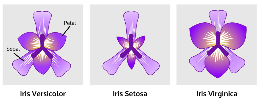
Figura 1. Flores de Iris. Disponibles en: Kaggle
Propiedad |
Valor |
Explicación |
|---|---|---|
Clases |
3 |
Las especies de iris: setosa, versicolor y virginica. |
Muestras por clase |
50 |
Cada especie tiene 50 flores |
Muestras totales |
150 |
3 clases × 50 muestras |
Dimensionalidad |
4 |
Cada flor tiene 4 características numéricas. |
Características |
Reales, positivas |
Todas las variables (longitud y ancho de sépalo y pétalo) son valores reales y positivos (no hay negativos). |
#datos
# Asigna las variables en X
X = datos['data'][:, 0:2].astype(int)
# Asigna las variables en y
y = datos['target']
y
array([0, 0, 0, 0, 0, 0, 0, 0, 0, 0, 0, 0, 0, 0, 0, 0, 0, 0, 0, 0, 0, 0,
       0, 0, 0, 0, 0, 0, 0, 0, 0, 0, 0, 0, 0, 0, 0, 0, 0, 0, 0, 0, 0, 0,
       0, 0, 0, 0, 0, 0, 1, 1, 1, 1, 1, 1, 1, 1, 1, 1, 1, 1, 1, 1, 1, 1,
       1, 1, 1, 1, 1, 1, 1, 1, 1, 1, 1, 1, 1, 1, 1, 1, 1, 1, 1, 1, 1, 1,
       1, 1, 1, 1, 1, 1, 1, 1, 1, 1, 1, 1, 2, 2, 2, 2, 2, 2, 2, 2, 2, 2,
       2, 2, 2, 2, 2, 2, 2, 2, 2, 2, 2, 2, 2, 2, 2, 2, 2, 2, 2, 2, 2, 2,
       2, 2, 2, 2, 2, 2, 2, 2, 2, 2, 2, 2, 2, 2, 2, 2, 2, 2])
print(len(X))
print(len(y))
150
150
# Genera un dataframe que integre X e y
df = pd.DataFrame(data=X,
                  columns=datos['feature_names'][:2])
df['y'] = y
df
| sepal length (cm) | sepal width (cm) | y | |
|---|---|---|---|
| 0 | 5 | 3 | 0 |
| 1 | 4 | 3 | 0 |
| 2 | 4 | 3 | 0 |
| 3 | 4 | 3 | 0 |
| 4 | 5 | 3 | 0 |
| ... | ... | ... | ... |
| 145 | 6 | 3 | 2 |
| 146 | 6 | 2 | 2 |
| 147 | 6 | 3 | 2 |
| 148 | 6 | 3 | 2 |
| 149 | 5 | 3 | 2 |
150 rows × 3 columns
help(df.rename)
Help on method rename in module pandas.core.frame:

rename(
    mapper: 'Renamer | None' = None,
    *,
    index: 'Renamer | None' = None,
    columns: 'Renamer | None' = None,
    axis: 'Axis | None' = None,
    copy: 'bool | lib.NoDefault' = <no_default>,
    inplace: 'bool' = False,
    level: 'Level | None' = None,
    errors: 'IgnoreRaise' = 'ignore'
) -> 'DataFrame | None' method of pandas.DataFrame instance
    Rename columns or index labels.

    Function / dict values must be unique (1-to-1). Labels not contained in
    a dict / Series will be left as-is. Extra labels listed don't throw an
    error.

    See the :ref:`user guide <basics.rename>` for more.

    Parameters
    ----------
    mapper : dict-like or function
        Dict-like or function transformations to apply to
        that axis' values. Use either ``mapper`` and ``axis`` to
        specify the axis to target with ``mapper``, or ``index`` and
        ``columns``.
    index : dict-like or function
        Alternative to specifying axis (``mapper, axis=0``
        is equivalent to ``index=mapper``).
    columns : dict-like or function
        Alternative to specifying axis (``mapper, axis=1``
        is equivalent to ``columns=mapper``).
    axis : {0 or 'index', 1 or 'columns'}, default 0
        Axis to target with ``mapper``. Can be either the axis name
        ('index', 'columns') or number (0, 1). The default is 'index'.
    copy : bool, default False
        This keyword is now ignored; changing its value will have no
        impact on the method.

        .. deprecated:: 3.0.0

            This keyword is ignored and will be removed in pandas 4.0. Since
            pandas 3.0, this method always returns a new object using a lazy
            copy mechanism that defers copies until necessary
            (Copy-on-Write). See the `user guide on Copy-on-Write
            <https://pandas.pydata.org/docs/dev/user_guide/copy_on_write.html>`__
            for more details.

    inplace : bool, default False
        Whether to modify the DataFrame rather than creating a new one.
        If True then value of copy is ignored.
    level : int or level name, default None
        In case of a MultiIndex, only rename labels in the specified
        level.
    errors : {'ignore', 'raise'}, default 'ignore'
        If 'raise', raise a `KeyError` when a dict-like `mapper`, `index`,
        or `columns` contains labels that are not present in the Index
        being transformed.
        If 'ignore', existing keys will be renamed and extra keys will be
        ignored.

    Returns
    -------
    DataFrame or None
        DataFrame with the renamed axis labels or None if ``inplace=True``.

    Raises
    ------
    KeyError
        If any of the labels is not found in the selected axis and
        "errors='raise'".

    See Also
    --------
    DataFrame.rename_axis : Set the name of the axis.

    Examples
    --------
    ``DataFrame.rename`` supports two calling conventions

    * ``(index=index_mapper, columns=columns_mapper, ...)``
    * ``(mapper, axis={'index', 'columns'}, ...)``

    We *highly* recommend using keyword arguments to clarify your
    intent.

    Rename columns using a mapping:

    >>> df = pd.DataFrame({"A": [1, 2, 3], "B": [4, 5, 6]})
    >>> df.rename(columns={"A": "a", "B": "c"})
       a  c
    0  1  4
    1  2  5
    2  3  6

    Rename index using a mapping:

    >>> df.rename(index={0: "x", 1: "y", 2: "z"})
       A  B
    x  1  4
    y  2  5
    z  3  6

    Cast index labels to a different type:

    >>> df.index
    RangeIndex(start=0, stop=3, step=1)
    >>> df.rename(index=str).index
    Index(['0', '1', '2'], dtype='str')

    >>> df.rename(columns={"A": "a", "B": "b", "C": "c"}, errors="raise")
    Traceback (most recent call last):
    KeyError: ['C'] not found in axis

    Using axis-style parameters:

    >>> df.rename(str.lower, axis="columns")
       a  b
    0  1  4
    1  2  5
    2  3  6

    >>> df.rename({1: 2, 2: 4}, axis="index")
       A  B
    0  1  4
    2  2  5
    4  3  6
# Renombra las columnas [length y width]
df.rename({'sepal length (cm)': 's_length',
           'sepal width (cm)': 's_width'},
           axis=1,
           inplace=True)
df.columns
Index(['s_length', 's_width', 'y'], dtype='str')
# Genera un conteo por tipo de flor
df['y'].value_counts()
y
0    50
1    50
2    50
Name: count, dtype: int64
Tipo de flor |
Número |
|---|---|
Setosa |
0 |
Versicolor |
1 |
Virginica |
2 |
📊
np.random.seed(1)
fig, ax = plt.subplots(figsize=(8, 6))
sc = ax.scatter( df.length + np.random.normal(loc=0, scale=0.1, size=len(df)), df.width + np.random.normal(loc=0, scale=0.1, size=len(df)), c=df.target, cmap=”cividis”, alpha=0.6, edgecolors=”w”, linewidths=0.5, s=60 )
ax.set_xlabel(«Sepal length (cm)», fontsize=12) ax.set_ylabel(«Sepal width (cm)», fontsize=12) ax.set_title(«Clasificación por longitud y ancho del sépalo», fontsize=14, pad=15)
ax.grid(True, linestyle=”–”, alpha=0.3)
cbar = fig.colorbar(sc, ax=ax) cbar.set_label(“Clase”, fontsize=11)
plt.tight_layout() plt.show()
# Gráfica
import numpy as np
np.random.seed(1)

fig, ax = plt.subplots(figsize=(8, 6))

sc = ax.scatter(
    df.s_length + np.random.normal(loc=0, scale=0.1, size=len(df)),
    df.s_width + np.random.normal(loc=0, scale=0.1, size=len(df)),
    c=df.y,
    cmap='cividis',
    alpha=0.6,
    edgecolors='w',
    linewidths=0.5,
    s=60
)


ax.set_xlabel("s_length", fontsize=12)
ax.set_ylabel("s_width", fontsize=12)
ax.set_title("Clasificación por longitud y ancho del sépalo", fontsize=14, pad=15)

ax.grid(True, linestyle='--', alpha=0.3)

cbar = fig.colorbar(sc, ax=ax)
cbar.set_label('Clase', fontsize=11)

plt.tight_layout()
plt.show()
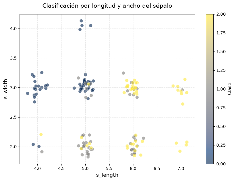
¿qué observamos?#
🧿
Clase 0 (color azul oscuro) está bien separada: se agrupa con sépalos más cortos y más anchos.
Clase 1 y Clase 2 (gris y amarillo) están más superpuestas, especialmente en la región de sépalos largos y estrechos.
Esto sugiere que, al menos con las variables
sepal lengthysepal width, la clase 0 se puede clasificar con mayor precisión que las otras dos.
Pregunta:
¿Cuáles modelos de clasificación podríamos usar para resolver este problema?
from sklearn.model_selection import train_test_split
from sklearn.tree import DecisionTreeClassifier
help(train_test_split)
Help on function train_test_split in module sklearn.model_selection._split:

train_test_split(
    *arrays,
    test_size=None,
    train_size=None,
    random_state=None,
    shuffle=True,
    stratify=None
)
    Split arrays or matrices into random train and test subsets.

    Quick utility that wraps input validation,
    ``next(ShuffleSplit().split(X, y))``, and application to input data
    into a single call for splitting (and optionally subsampling) data into a
    one-liner.

    Read more in the :ref:`User Guide <cross_validation>`.

    Parameters
    ----------
    *arrays : sequence of indexables with same length / shape[0]
        Allowed inputs are lists, numpy arrays, scipy-sparse
        matrices or pandas dataframes.

    test_size : float or int, default=None
        If float, should be between 0.0 and 1.0 and represent the proportion
        of the dataset to include in the test split. If int, represents the
        absolute number of test samples. If None, the value is set to the
        complement of the train size. If ``train_size`` is also None, it will
        be set to 0.25.

    train_size : float or int, default=None
        If float, should be between 0.0 and 1.0 and represent the
        proportion of the dataset to include in the train split. If
        int, represents the absolute number of train samples. If None,
        the value is automatically set to the complement of the test size.

    random_state : int, RandomState instance or None, default=None
        Controls the shuffling applied to the data before applying the split.
        Pass an int for reproducible output across multiple function calls.
        See :term:`Glossary <random_state>`.

    shuffle : bool, default=True
        Whether or not to shuffle the data before splitting. If shuffle=False
        then stratify must be None.

    stratify : array-like, default=None
        If not None, data is split in a stratified fashion, using this as
        the class labels.
        Read more in the :ref:`User Guide <stratification>`.

    Returns
    -------
    splitting : list, length=2 * len(arrays)
        List containing train-test split of inputs.

        .. versionadded:: 0.16
            If the input is sparse, the output will be a
            ``scipy.sparse.csr_matrix``. Else, output type is the same as the
            input type.

    Examples
    --------
    >>> import numpy as np
    >>> from sklearn.model_selection import train_test_split
    >>> X, y = np.arange(10).reshape((5, 2)), range(5)
    >>> X
    array([[0, 1],
           [2, 3],
           [4, 5],
           [6, 7],
           [8, 9]])
    >>> list(y)
    [0, 1, 2, 3, 4]

    >>> X_train, X_test, y_train, y_test = train_test_split(
    ...     X, y, test_size=0.33, random_state=42)
    ...
    >>> X_train
    array([[4, 5],
           [0, 1],
           [6, 7]])
    >>> y_train
    [2, 0, 3]
    >>> X_test
    array([[2, 3],
           [8, 9]])
    >>> y_test
    [1, 4]

    >>> train_test_split(y, shuffle=False)
    [[0, 1, 2], [3, 4]]

    >>> from sklearn import datasets
    >>> iris = datasets.load_iris(as_frame=True)
    >>> X, y = iris['data'], iris['target']
    >>> X.head()
        sepal length (cm)  sepal width (cm)  petal length (cm)  petal width (cm)
    0                5.1               3.5                1.4               0.2
    1                4.9               3.0                1.4               0.2
    2                4.7               3.2                1.3               0.2
    3                4.6               3.1                1.5               0.2
    4                5.0               3.6                1.4               0.2
    >>> y.head()
    0    0
    1    0
    2    0
    3    0
    4    0
    ...

    >>> X_train, X_test, y_train, y_test = train_test_split(
    ... X, y, test_size=0.33, random_state=42)
    ...
    >>> X_train.head()
        sepal length (cm)  sepal width (cm)  petal length (cm)  petal width (cm)
    96                 5.7               2.9                4.2               1.3
    105                7.6               3.0                6.6               2.1
    66                 5.6               3.0                4.5               1.5
    0                  5.1               3.5                1.4               0.2
    122                7.7               2.8                6.7               2.0
    >>> y_train.head()
    96     1
    105    2
    66     1
    0      0
    122    2
    ...
    >>> X_test.head()
        sepal length (cm)  sepal width (cm)  petal length (cm)  petal width (cm)
    73                 6.1               2.8                4.7               1.2
    18                 5.7               3.8                1.7               0.3
    118                7.7               2.6                6.9               2.3
    78                 6.0               2.9                4.5               1.5
    76                 6.8               2.8                4.8               1.4
    >>> y_test.head()
    73     1
    18     0
    118    2
    78     1
    76     1
    ...
# Genera un clasificador de árbol de decisión
X_train, X_test, y_train, y_test = train_test_split(X, y, test_size=0.1, random_state=42)
# Predicciones
ml_clf = DecisionTreeClassifier(max_depth=1)
ml_clf.fit(X_train, y_train)
DecisionTreeClassifier(max_depth=1)In a Jupyter environment, please rerun this cell to show the HTML representation or trust the notebook.
On GitHub, the HTML representation is unable to render, please try loading this page with nbviewer.org.
Parameters
Fitted attributes
# y_pred
y_pred = ml_clf.predict(X_test)
# y_pred
y_pred
array([2, 0, 2, 2, 2, 0, 0, 2, 2, 0, 2, 0, 0, 0, 0])
# y_test
y_test
array([1, 0, 2, 1, 1, 0, 1, 2, 1, 1, 2, 0, 0, 0, 0])
# y_pred == y_test (máscara booleana)
mask = y_pred == y_test
# promedio de aciertos con y_test
mask.mean()
np.float64(0.6)
¿Por qué usar una distribución conjunta para clasificar?#
Anteriormente vimos que un modelo de clasificación (como árboles de decisión) presenta un score del 60%.
Podemos adoptar un enfoque probabilístico para modelar la situación a partir de los datos disponibles.
# Convierte en df los datos de train
train_df = pd.DataFrame(data=X_train,
                        columns=['L', 'W'])
train_df['T'] = y_train
train_df
| L | W | T | |
|---|---|---|---|
| 0 | 6 | 3 | 1 |
| 1 | 6 | 3 | 2 |
| 2 | 5 | 2 | 1 |
| 3 | 5 | 2 | 1 |
| 4 | 6 | 2 | 2 |
| ... | ... | ... | ... |
| 130 | 6 | 2 | 1 |
| 131 | 4 | 2 | 2 |
| 132 | 5 | 4 | 0 |
| 133 | 5 | 2 | 1 |
| 134 | 7 | 3 | 2 |
135 rows × 3 columns
# Convierte en df los datos de test
test_df = pd.DataFrame(data=X_test,
                       columns=['L', 'W'])
test_df['T'] = y_test
test_df
| L | W | T | |
|---|---|---|---|
| 0 | 6 | 2 | 1 |
| 1 | 5 | 3 | 0 |
| 2 | 7 | 2 | 2 |
| 3 | 6 | 2 | 1 |
| 4 | 6 | 2 | 1 |
| 5 | 5 | 3 | 0 |
| 6 | 5 | 2 | 1 |
| 7 | 6 | 3 | 2 |
| 8 | 6 | 2 | 1 |
| 9 | 5 | 2 | 1 |
| 10 | 6 | 3 | 2 |
| 11 | 4 | 3 | 0 |
| 12 | 5 | 3 | 0 |
| 13 | 4 | 3 | 0 |
| 14 | 5 | 3 | 0 |
# Imprime los valores únicos de L, W y T
print(train_df['L'].nunique())
print(train_df['W'].nunique())
print(train_df['T'].nunique())
4
3
3
Primero, veámos en la tabla siguiente que las columnas (L, W T) representan todas las posibles combinaciones de valores de cada variable.
La tabla muestra la distribución conjunta de tres variables (L, W, T).
Al estimar la distribución conjunta de las variables \((L)\) (longitud del tallo), \((W)\) (ancho del tallo) y \((T)\) (tipo de flor), obtenemos un modelo probabilístico completo:
Este enfoque tiene varias ventajas:
Captura todas las relaciones entre las variables.
Nos permite derivar distribuciones condicionales útiles para clasificación.
# Generamos un conteo relativo (para construir la distribución empírica)
train_df.groupby(['L', 'W', 'T']).size()
L  W  T
4  2  0     2
      1     1
      2     1
   3  0    16
5  2  1    17
      2     5
   3  0    22
      1     6
      2     1
   4  0     4
6  2  1    10
      2    11
   3  1     9
      2    18
7  2  2     3
   3  1     1
      2     8
dtype: int64
Tenemos \(4 * 3 * 3 = 36\) posibles combinaciones:
NOTA: no todas las combinaciones posibles de (L, W T) aparecen en los datos. groupby().size() solo muestra las combinaciones que realmente están presentes en el DataFrame.
Las combinaciones que no ocurren ni una sola vez, no aparecen en la salida porque su conteo es \(0\).
L |
W |
T |
Frecuencia |
|---|---|---|---|
4 |
2 |
0 |
2 |
4 |
2 |
1 |
1 |
4 |
2 |
2 |
1 |
4 |
3 |
0 |
16 |
5 |
2 |
1 |
17 |
5 |
2 |
2 |
5 |
5 |
3 |
0 |
22 |
5 |
3 |
1 |
6 |
5 |
3 |
2 |
1 |
6 |
2 |
1 |
10 |
6 |
2 |
2 |
11 |
6 |
3 |
1 |
9 |
6 |
3 |
2 |
18 |
7 |
2 |
2 |
3 |
7 |
3 |
1 |
1 |
7 |
3 |
2 |
8 |
# Generamos la distribución empírica conjunta (conteo/normalización)
empirical_joint_distr = train_df.groupby(['L', 'W', 'T']).size() / len(train_df)
empirical_joint_distr
L  W  T
4  2  0    0.014815
      1    0.007407
      2    0.007407
   3  0    0.118519
5  2  1    0.125926
      2    0.037037
   3  0    0.162963
      1    0.044444
      2    0.007407
   4  0    0.029630
6  2  1    0.074074
      2    0.081481
   3  1    0.066667
      2    0.133333
7  2  2    0.022222
   3  1    0.007407
      2    0.059259
dtype: float64
# ¿la distribución empírica conjunta suma 1?
empirical_joint_distr.sum()
np.float64(1.0)
#
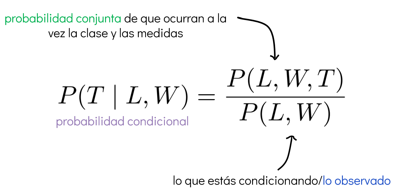
Por ejemplo, a partir de la distribución conjunta podemos obtener la probabilidad de que una flor pertenezca a cierta clase \((T)\), dado que observamos un par de medidas \(((L, W))\):
Con esta información, podemos construir un clasificador probabilístico de la siguiente manera:
La distribución condicional nos proporciona una probabilidad para cada posible valor \((t)\) que puede tomar la variable \((T)\) (por ejemplo, \((t = 0, 1, 2 )\)). Como nuestro objetivo es predecir la clase más probable, elegimos el valor de \((t)\) que maximiza esta probabilidad:
Este procedimiento se conoce como el clasificador MAP (Maximum A Posteriori). Es importante destacar que no necesitamos calcular explícitamente la distribución condicional, ya que:
Dado que el denominador \((P(L = \ell, W = w))\) no depende de \((t)\), podemos omitirlo durante la maximización. Esto nos permite simplificar el clasificador a:
Este enfoque nos permite realizar clasificación directamente a partir de la distribución conjunta estimada, sin necesidad de modelos adicionales.
# empirical_joint_distr[7, 3].idxmax()
empirical_joint_distr.loc[(5, 3)].idxmax()
np.int64(0)
# Generar por a partir de la distribución emírica el argmax
pred = []

for _, row in test_df.iterrows():
    pred.append(empirical_joint_distr[(row['L'], row['W'])].idxmax())

y_pred_prob = np.array(pred)
y_pred_prob
array([2, 0, 2, 2, 2, 0, 1, 2, 2, 1, 2, 0, 0, 0, 0])
# y_test
y_test
array([1, 0, 2, 1, 1, 0, 1, 2, 1, 1, 2, 0, 0, 0, 0])
# promedio de aciertos con y_test
mask = y_pred_prob == y_test
mask.mean()
np.float64(0.7333333333333333)
📌 Conclusión#
Pasos que seguiste (en términos probabilísticos)
Estimación de la distribución conjunta
Calculaste la probabilidad conjunta \((P(L = \ell, W = w, T = t))\) a partir de los datos, contando la frecuencia de cada combinación y normalizando sobre el total.
Normalización
Dividiste los conteos conjuntos por el total de observaciones, obteniendo así una estimación empírica de las probabilidades.
→ Esto convierte los conteos en una distribución de probabilidad válida.Cálculo de la probabilidad condicional
usaste la regla de Bayes para pasar de probabilidades conjuntas a probabilidades condicionales:
\[ P(T = t \mid L = \ell, W = w) = \frac{P(L = \ell, W = w, T = t)}{P(L = \ell, W = w)} \]Predicción con argumento máximo (MAP)
Elegiste la clase con mayor probabilidad condicional:
\[ \hat{t} = \arg\max_t P(T = t \mid L = \ell, W = w) \]→ Esto significa que, dadas las evidencias (los valores de \(L\) y \(W\)), escoges la clase más plausible según los datos observados.
Clasificación final
Aplicaste este procedimiento a cada punto del conjunto de datos, generando predicciones basadas únicamente en la distribución conjunta estimada.
OJO
Que ambos modelos obtengan el mismo score no significa que sean equivalentes, sino que dado el conjunto de datos y la tarea, ambos llegaron al límite razonable de desempeño.
Ambos tienen ventajas:
El modelo probabilístico aporta una visión basada en evidencia y probabilidades.
El árbol de decisión proporciona reglas claras y visualmente interpretables.